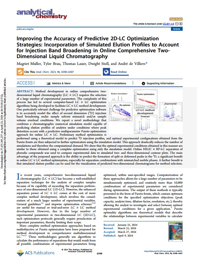
Improving the Accuracy of Predictive 2D-LC Optimization Strategies: Incorporation of Simulated Elution Profiles to Account for Injection Band Broadening in Online Comprehensive TwoDimensional Liquid Chromatography
Posting date on solidfuturism: May 2th 2024
Published date: March 27th 2024
Authors: Magriet Muller, Tyler Brau, Thomas Lauer, Dwight Stoll, and André de Villiers
DOI: 10.1021/acs.analchem.4c00491
Abstract composer: Seyed Amirhosein Mirsadri
Nowadays, the use of High-Performance Liquid Chromatography (HPLC) is very common among chemists. There is a type of this device that offers unique capabilities to chemists, which is nothing other than two-dimensional chromatography (LC×LC). This means that the output of the first chromatography enters the input of the second chromatography. In this case, the phases and polarity of the columns of the two chromatography devices may be very different, which makes optimizing the device for separation more complicated. This is because the parameters affecting the optimization of high-efficiency separation increase exponentially. Today, scientists use simulation methods before testing with the device and reach the most optimal states with calculations of different states and mathematical formulas. This method, called the Pareto Algorithm, can find many commonalities between different real experiments with theoretical models and use them in its calculations, and ultimately show the resolution and peak capacity of the chromatogram accurately. However, there was a problem with the time-consuming nature of the calculations, which could continue for days with an increase in parameters (depending on the type of computer). Therefore, this article has tried to perform faster and higher quality simulations by defining a new mathematical model for "injection band broadening" problems. This model uses Craig counter-current flow distribution equations to simulate the interaction of two phases inside the chromatography column using asymmetric injection profiles that benefit from the two-dimensional chromatography injection valve to improve simulation accuracy.

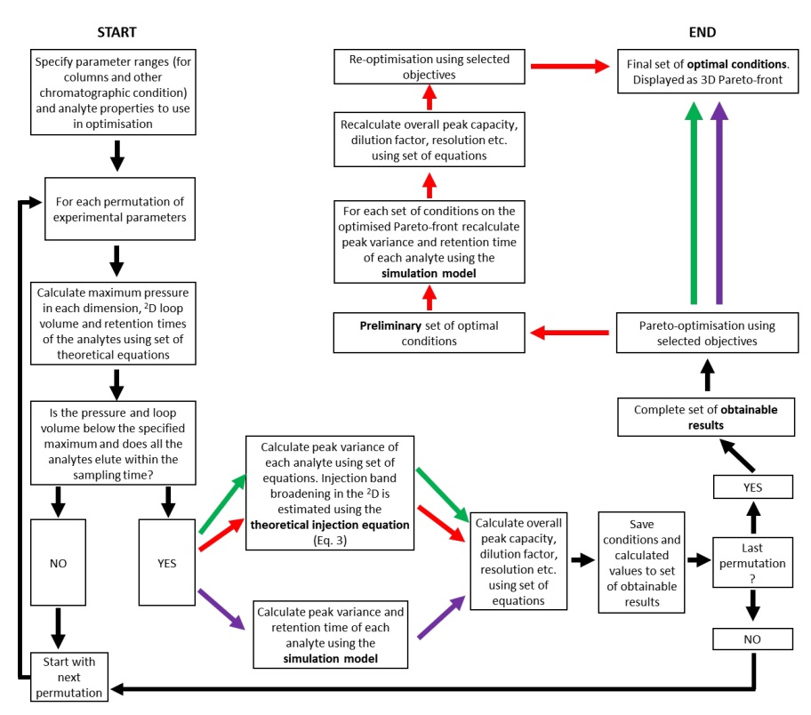
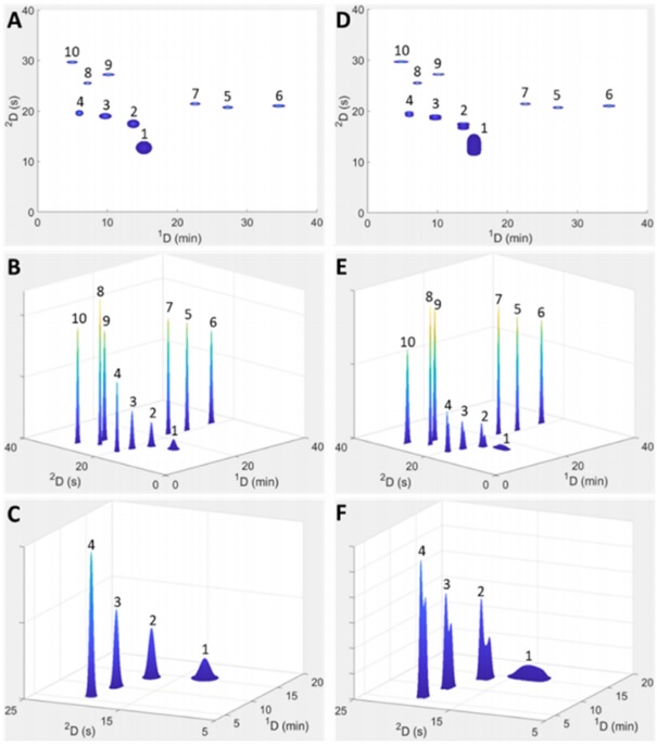
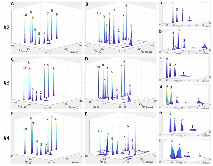
The input parameters required for this method include the height of theoretical plates, retention times, and column characteristics (porosity, flow resistance, column length, column diameter, particle size). Optimization equations are usually drawn and described in three-dimensional diagrams. Also, in this study, three equations have been used to extract data for optimization in three cases. The theoretical injection equation for peak broadening due to injection, the second equation is numerical simulation equations for solvent ratio values and sample dilution, and numerical simulation equations for the Pareto algorithm have been used. These calculations were performed on the Amaron cloud computer using MATLAB software. Many phenol-containing samples were prepared to be examined with Pareto pattern simulations, Craig model, and real experiments. In these experiments, it was found that the newer algorithm, which was much faster, showed results consistent with the previous slow algorithm, as each simulation showed very good compatibility with the results and real experiments. The only difference was that the simulation diagrams had cleaner peaks and lacked background.

However, the new model was able to add a feature to the previous capabilities, which was that sometimes the peak diagrams showed bifurcation. Peak bifurcation can generally be a reason for the analyte's incompatibility with the column, or the analyte's retention in the column, or additional peak broadening problems due to injection, which usually occurs in two-dimensional devices where one column device has opposite polarity to the next device. Therefore, we can detect it before injection into the column and refrain from doing so. These calculations were performed on the Amaron cloud system for 324 hours, although the peak broadening in reality was much more than what was simulated. The reasons for these differences can be attributed to the continuous change in the internal radial temperature gradient of the column resulting from friction and the flow of the injection module valve before the column (in calculations, more attention has been paid to the characteristics and events after the column). Therefore, this article was able to present a new and faster model for simulating the optimization of two-dimensional high-performance liquid chromatography.


klsjuidhfasdgh.png)
klsjuidhfasdgh.png)
klsjuidhfasdgh.png)
klsjuidhfasdgh.png)
klsjuidhfasdgh.png)

klsjuidhfasdgh.png)
klsjuidhfasdgh.png)
klsjuidhfasdgh.png)